
Science and mathematics progress by degrees, sometimes by massive leaps. The progression is not something that you can know looking forward, it must be understood looking backward. Nor is progress necessarily linear. This holds true especially in our time of massive computation and parallelization. As progress conforms more to super linear laws, our ability to track it decreases. Yet we still desire to understand how far we’ve come.
A process cannot be understood by stopping it. Understanding must move with the flow of the process, must join it and flow with it. - Frank Herbert, Dune
To this end, Andrew Gelman and Aki Vehtari published an important paper in 2021. The paper reviews 8 ideas that represent broad categories of statistics and machine learning that have had major advancements made in the last 50 years. I wanted to include a review of the review. I’ll add a little color of my own and expand with more examples and visuals. If only you develop a better appreciation for the rapid pace of change in our field, that will be enough. Discussing the common threads is very important too, as the developments are many but the common threads are much fewer. Finally, there is one massive development that has occurred since the paper was published (see if you can guess what it is), so we’ll discuss that as well.
Counterfactual Causal Inference
Prediction is often what we seek when we build models. Causality takes it a step further from association to causal links, levers that can be manipulated in the data generating process. The past 50 years has been an absolute gold mine for the development of causal techniques that ground causality in a scientific framework. Below we discuss two of the most important sub fields.
Potential Outcomes
Previously, the field of statistics had a loose relationship with causality. Most of the time we relied on Randomized Controlled Trials and didn’t deal with heterogenous effects. Early on the arenas of descriptive and causal, or rather associative and causal, were not properly teased out. That all changed with the introduction of formalities around counterfactuals and the potential outcomes framework. Counterfactuals are where we imagine a world of events that never happened, and calculate this outcome if things had gone differently. The most basic example is the case of drug treatment. For a given individual, you cannot receive treatment and non-treatment at the same time. We have to generate the counterfactual world where you didn’t receive treatment and compare that to the real world where you did to see if the drug has efficacy. Potential outcomes put this formulation into solid theoretical and practical territory. That counterfactual inference wasn’t put on steady legs sooner is surprising given the similarities in abstraction between hypothesis testing and counterfactuals. Both posit two different worlds for comparison to come to an insight about the true nature of a parameter. In both, one exists and the other doesn’t. No matter, how can you learn more about these developments? Rubin, Pearl, and Athey are the biggest names in this space, so check out their work for more information.

Causal Discovery
Causal discovery (CD) is an exciting area of research in Causal inference that will yield tremendous benefits in the future for the field of statistics. The idea is that given a dataset where you either don’t know the causal mechanisms or you want to verify a hypothesis, you can utilize causal discovery techniques to generate one or more causal graphs for the data generating process. The underlying algorithms seek out statistical dependencies between the data in addition to confounders that obscure causal relationships. Remember, association doesn’t necessarily mean causation, but if there is no association (statistical dependency), then there is no causal link.
Some of the available techniques of CD include
- Conditional Indepedence Testing
- Greedy Search of DAG Space
- Assymetry based
- Hybrid Approach
Let’s describe one algorithm belonging to the Conditional Independence bucket to motivate further study and illustrate how this process could work.
The algorithm is called the PC algorithm. The steps are roughly as follows
- Form a fully connected graph using all available features in the dataset
- Eliminate edges (connections) between features that are statistically independent
- Test for conditional dependencies using the remaining edges
- Create separation sets for variables if a conditioning variable removes dependencies between those variables
- Orient colliders using the Separation sets
- Using constraints (no new colliders and no cycles), complete the graph
The Greedy Equivalence Search (GES) is the exact opposite, start with a graph where there are no edges between variables and greedily add edges that increase the model fitness score. There are many packages that give access to programmatic implementations of these algorithms, consider starting here if you’re interested.
Boostrap and simulation
Much of what we’re doing when we use statistics beyond basic descriptives is to estimate the sampling distribution of a parameter of the population. Oftentimes, when assumptions are met, we have closed formed methods to calculate these statistics very quickly. A major trend in statistics, and a common theme of this article, is to replace this mathematical estimation in favor of estimation based on raw computing. The bootstrap is the most ubiquitous method that takes this approach. The bootstrap takes advantage of the rise of computing power (see Moore’s Law) to estimate the parameter of interest by multiple runs of resampling. This can also be used in a modeling pipeline too, where new datasets are generated from a model instead of an original dataset.
Imagine you can’t meet assumptions of the particular model you want to use, or you are comparing statistics in two distributions that are not identical. Bootstrap is your friend. There is a lot of similarity with the bagging approach used in ensembles to reduce variance, only we are trying to characterize variance with the bootstrap, not mimimize it.
Another common application is to obtain robust inference around feature importances in model evaluation. For example in Random Forests, you can obtain point estimates for model feature importances readily, but have no way to tell if they are significant or stable. Permuting the model, say by scrambling or removing a feature multiple times, and generating a sampling distribution not only allows you to circumvent having to know the true distribution, but it allows you to assess the significance of the estimate using measures that are well understood like standard error or confidence intervals.
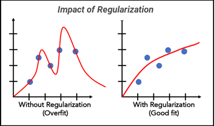
Overparameterized Models and Regularization
The Bias-Variance tradeoff and the Curse of dimensionality are the inescapable realities of statistical modeling. They are fundamental to everything that happens in our field. Early on in statistical sciences, the data available was small in both the sense that there were fewer datapoints and that the number of features was limited too. This has changed and and this change leads to overparamatrized models, where the available features sometimes can even exceed the number of datapoints. In high dimenionsal data spaces, this results in incredible sparsity in the search space introduces variance into model predictions. Perhaps we don’t want to discard the rich feature set we’ve obtained, but we also need stable estimates. In comes Regularization, along with other methods like Model Stacking, Bagging, Boosting, Lasso, SVMs, and many other techniques that allow us to do just that. Regularization allows us to achieve stability in our model outputs while still retaining our rich feature set. It does so by introducing bias into our model, in favor of a reduction in variance. That’s why it’s called a tradeoff. Note that when you use regularization on an OLS model, it is no longer BLUE, but may have a lower Mean Squared Error (MSE) than the unbiased model. So practically, caution should be used if you’re combining say causal modeling with Ridge regression (OLS plus regularization), since the model parameters will be biased on purpose. I won’t say more other than to suggest that you use these techniques liberally in your model when it makes sense to, and that you learn through experience.
Bayesian Multilevel Models (BMLMs)
We know in this complex world, many factors influence outcomes. Sometimes these factors do not exist on the same level of abstraction as others. How do we incorporate them all into our models?
BMLMs can solve this problem. The fundamental principle of BMLMs is to represent the data as emerging from different levels of variation. For instance, in a study of students’ test results, the individual scores may be modeled as a function of both individual-level and group-level factors, such as past knowledge or the student’s school or teacher. The individual-level variables reflect differences in performance between students within a specific school or teacher, whereas the group-level variables capture performance differences between schools or teachers. Another example would be modeling stock prices, where a stock’s movement depends on both the fundamentals of the company and the broader market conditions, which are clearly different concerns. A rising tide raises all ships.
How can we estimate these BMLMs? Markov chain Monte Carlo (MCMC) simulation, a Bayesian computing technique, is a popular method for fitting BMLMs. To estimate the posterior mean, variance, and credible intervals of the model parameters, MCMC creates samples from the posterior distribution of the model parameters. More on MCMC in python here
All things considered, BMLMs offer an adaptable framework for modeling complicated data with both individual and group-level variance. In disciplines like social science, psychology, and education, where data frequently reveal complicated hierarchical structures, BMLMs are extensively used.
Generic Computation Algorithms
This is an interesting section in that it represents the influence of another field on statistics. Crossover leads to new developments in a field and stats is no different. If you want to speed up the total rate of computation, you have several methods available. One is to speed up the underlying hardware by creating more transistors on your chip or providing more RAM. Another way is to find a more efficient algorithm.
Some of the algorithms that have had an impact on statistics include Gradient Descent, Singular Value Decomposition, and Randomized Algos (like MCMC). Efficient algorithms have an outsized contribution to advances in Bayesian statistics, where the distributions you want to calculate cannot be computed quickly but must rather be sampled from to estimate. More efficient algorithms such as Gibb’s Sampling led to more uptake in the use of Bayesian techniques, where the mathematics were solid but computing time was too long for widespread adoption. Most recently, Fourier Analyses have been suggested for use to understand how neural networks come about their predictions in a physical science domain
This importance of the underlying algorithms also plays into the language wars we see being waged between statistical languages like python and R. Both are relatively slow when compared across basic tasks with lower level languages like C. However they increase efficiency in that it’s easier to write the same code in python than it is in the low level languages where you have to perform memory management and declare types. This shows a meta perspective on efficiency, where algo efficiency is only one dimension. To motivate the discussion further, here are two more points that hopefully will show you why you should care. I’m not saying that data scientists and statisticians should learn how to sort a binary tree necessarily, but at a minimum we should understand how algorithmic developments have enabled the work we do now.
- Solve it or don’t - Using Big O notation, if you have a problem that can be solved by two algos, one which is O(n log n) and another which is O(n^3), the latter may never complete in the lifetime of the user, while the former is the time complexity of many sorting algorithms. This illustrates the difference between solving the problem and not solving it at all. When computing parameters on high dimensional distributions, you need efficient algorithms to go from 0 to 1.
- The move to the cloud - Many analytics type workflows take place on the cloud now. With pricing models similar to AWS Lambda, where you pay only for compute that is used, it pays to have an efficient algorithm so that costs don’t get run up. Why analyze a sample when you can run your analysis on the entire population?
Adaptive Decision Analysis (ADA)
Adaptive decision analysis is an important field in artificial intelligence that involves developing decision-making systems that can learn and improve their performance over time. Bayesian optimization is a popular method for ADA that involves using Bayesian inference to optimize complex functions by iteratively selecting a new point to evaluate based on the previous observations. This method has been applied to a wide range of problems, including optimizing the performance of machine learning models and tuning hyperparameters. scikit-optimize is an implementation you may enjoy exploring
Reinforcement learning is another important technique in ADA that involves learning optimal behavior through trial and error (sounds familiar, eh programmers?). This technique has been successfully applied to a wide range of practical tasks, including game playing. For example, the game of Go has long been considered a challenging problem for AI due to the search space of possible moves being larger than the number of atoms in the universe. In 2016, the AlphaGo system, developed by Google DeepMind, defeated the world champion Lee Sedol at Go, demonstrating the power of reinforcement learning in developing adaptive decision-making systems.

Multi-armed bandits are another important class of problems, which involves balancing the exploration-exploitation tradeoff. In these problems, the decision-maker must balance between trying out new actions (exploration) and exploiting the currently known best action (exploitation). Multi-armed bandits have important applications in areas such as clinical trials, online advertising, and recommendation systems.
Robust Inference
Robustness is the idea that we can estimate parameters and models even in the case where there are violations of assumptions for the estimating process. Robust inference is vital to all of modern statistics, especially as the amount of data proliferates (at a rate of 2x every 2 years, a growth of 41% a year). It is unfair to think that the data generating process behind all of these phenomena will neatly meet the assumptions of OLS. This feeds directly into the reason that the bootstrap is a good estimator because it does not make any assumptions on the DGP and therefore provides us a level of robustness to violations.
The idea of robustness also plays into the desire to reduce variance in our model outputs. This can take many names, including High Variance models, model misspecification, or model dependence, but the underlying idea is the same. We do not wish for our estimates to change dramatically either when we slightly change the model (model dependence) or change up the input data to the model (model variance). Cross validation is a great way to reduce variance in estimates of model performance metrics, by varying up the input data enough that, asymptotically, your model should see close to the entirety of the sample space. Bagging also answers this by aggregating model estimates trained on different subsets of the original dataset that may or may not have been out of bag or bootstrapped.
Exploratory Data Analysis
This section was a bit surprising to me. The reason being that EDA is such an open ended process, and usually involves more creativity than anything, that it doesn’t seem that there should be major developments here. And yet it makes sense when you consider cultural changes. Statisticians used to view calculations as exact, and graphs as only rough add ons. Discovery vs testing fixed hypotheses, where they can be complementary. The authors highlight EDA in comparison to asymptotic theory as two modes of analysis in stats, and the comparison is revealing.
Asymptotic theory is important for inference, as it allows us to gain insights about the population based only on a sample. All of statistics exists because we don’t have omniscience and/or infinite resources. However, asymptotic theory is not always sufficient to fully understand the properties of a dataset, especially when the sample size is small or the data is non-normal or non-linear. One classic example is Anscombe’s quartet, which consists of four different datasets that have identical summary statistics, but very different distributions and patterns.

Asymptotic theory assumes that the sample size is large enough for the law of large numbers to hold, and that the distribution of the estimator converges to a normal distribution as the sample size approaches infinity. However, this assumption may not hold in small sample sizes or when the data is non-normally distributed. This is where exploratory data analysis (EDA) becomes important, as it allows us to visually inspect the data and identify patterns that may not be apparent through asymptotic theory. EDA helps to identify potential issues such as outliers, skewness, and non-linear relationships, which can help inform the choice of appropriate statistical methods for the data. In summary, while asymptotic theory is an important part of statistical inference, it is not always sufficient, and exploratory data analysis is a critical tool for identifying potential issues and guiding the appropriate statistical methodology for a given dataset.
The use of exploratory analysis also enhances ML model creation/evaluation. EDA can assist in locating patterns and trends in the data that can guide the creation of a machine learning model that is appropriate for the modeling task. To improve the performance of the model, EDA might, for instance, assist in locating any outliers or abnormalities in the data that could point to problems or imply the need for preprocessing or transformation activities. In order to make the best choice of features for the model, EDA can also assist in locating features that might have a strong link with the target variable. EDA can also aid in locating any confounding factors or interactions between elements that could influence the model’s performance, for example identifying collinear variables. Finally, all of the techniques of EDA are helpful in evaluating the model’s performance. If you want to evaluate multiple metrics simultaneously, or visualize the cross fold performance of a training classifier, EDA is your friend here. EDA should almost always be a part of your workflow, so it pays to become adept at it.
Even More Developments
While the original article is not very old, the pace of change has accelerated such that new developments have occurred since the article was published that almost certainly would have been mentioned
Large Language Models
Large Language Models (LLMs) have begun a new revolution in the AI space. What are they? Simply put, they are probability distributions for word sequences, trained on massive amounts of text obtained from openly available scripts, websites, books, anything containing text on the internet. These LLMs have converged on the Transformer architecture in the past few years. Check out this link to learn more about Transformers. Or you can use an LLM to explain it to you. LLMs are immediately useful out of the box after their initial training on input text, but can also add much more value when they are “fine tuned” on a narrower scope of text for a given domain. Given high quality prompts and responses within a niche domain, LLMs can become very powerful for solving problems in those domains. Transformer LLMs were around when the authors penned their article (see BERT), but perhaps the sweeping innovation that they are was not apparent to them at the time.
The most recent LLM that has generated buzz is the ChatGPT model developed by OpenAI. ChatGPT is a model that builds on the success of GPT-3 which came out around 2020. It delivers a chatbot like experience that has set the standard for all other LLMs, and simultaneously kicked off n model arms race that is difficult to keep track of. You can converse with it almost like you were talking to a human, where it emulates general knowledge (learned from the text sequences it was trained on) and can remember the context of a conversation. People, myself included, have found it to be incredibly helpful at generating new ideas for business, solve coding challenges, generate recipes, bounce ideas off, and so much more. For now, access to ChatGPT is completely free, but only because OpenAI is using each user’s interaction with the platform to further the development of the model.
At risk of beating this horse to death, one common theme of our article is that developments in computing have enabled further developments in statistics, and LLMs are no different. These models are currently so taxing to train or fine tune computationally that most people do not have access to enough computing power to manipulate these models directly on their own infrastructure. The training budget for ChatGPT is estimated to be in the millions of dollars. Most of us are used to having models train for a few minutes, if that, so it’s clear that we are undergoing a paradigm shift that pushes us even closer to the edge of our resources. With access to GPUs and TPUs, these models can be trained in a more efficient manner, taking advantage of the incredible ability for these hardware devices to quickly perform the matrix computations required to train the neural nets behind these models.
LLMs are set to disrupt nearly every industry. It is hard to think of one that won’t be affected. Many say that ChatGPT will make software developers and data scientists obsolete, but this is far from the case in the near term. As a wise person on Linkedin said, you won’t be replaced by AI, you’ll be replaced by a person using AI. I think they are right. The future, in the near term, is Human in the Loop. The beauty of this approach is that we can rely on computers to do what they are good at, and we continue to perform the tasks that play to our strengths, maximizing the benefit. But make no mistake, the ripple effects of this technology cannot be predicted. The only thing that we can predict is that it will transform everything. Ironic that the underlying models are called transformers. They will do just that.
If you are a crazy person and have your own personal GPU farm, or you just have money to blow, why not try fine tuning the Bloom model to your specific domain? If you do this, reach out and let me know how it goes.
Until next time.
#statistics #ml